Using R as a GIS

In real estate, spatial data is the name of the game. Countless programs
in other domains utilize the power of this data, which is becoming more
prevalent by the day.

In this post I will go over a few simple, but powerful tools to get you
started using using geographic information in R.

##First, some libraries##
#install.packages('GISTools', dependencies = T)
library(GISTools)

GISTools provides an easy-to-use method for creating shading schemes
and choropleth maps. Some of you may have heard of the sp package,
which adds numerous spatial classes to the mix. There are also functions
for analysis and making things look nice.

Let’s get rolling: source the vulgaris dataset, which contains
location information for Syringa Vulgaris (the Lilac) observation
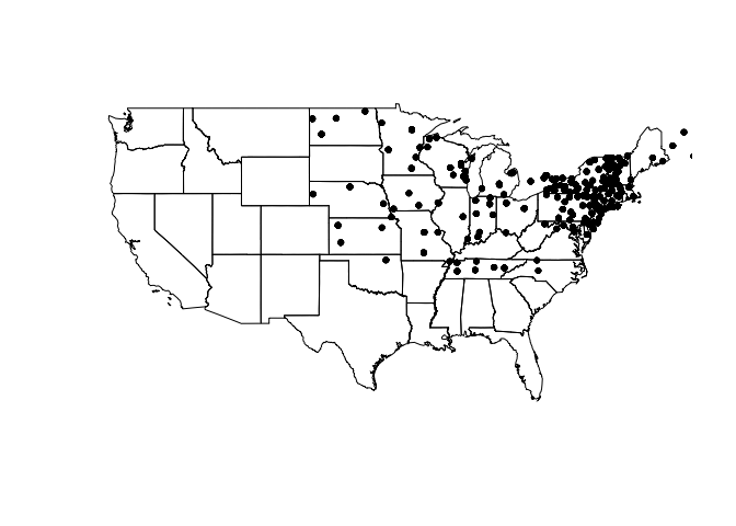
stations and US states. This code plots the states and vulgaris
points.

data("vulgaris") #load data
par = (mar = c(2,0,0,0)) #set margins of plot area
plot(us_states)
plot(vulgaris, add = T, pch = 20)

One thing to note here is the structure of these objects. us_states is
a SpatialPolygonsDataFrame, which stores information for plotting shapes
(like a shapefile) within its attributes. vulgaris by contrast is a
SpatialPointsDataFrame, which contains data for plotting individual
points. Much like a data.frame and $, these objects harbor
information that can be accessed via @.

kable(head(vulgaris@data))

	Station	Year	Type	Leaf	Bloom	Station.Name	State.Prov	Lat	Long	Elev
3695	61689	1965	Vulgaris	114	136	COVENTRY	CT	41.8	-72.35	146
3696	61689	1966	Vulgaris	122	146	COVENTRY	CT	41.8	-72.35	146
3697	61689	1967	Vulgaris	104	156	COVENTRY	CT	41.8	-72.35	146
3698	61689	1968	Vulgaris	97	134	COVENTRY	CT	41.8	-72.35	146
3699	61689	1969	Vulgaris	114	138	COVENTRY	CT	41.8	-72.35	146
3700	61689	1970	Vulgaris	111	135	COVENTRY	CT	41.8	-72.35	146

Let’s take a look at some functions that use this data.

newVulgaris kable(head(data.frame(newVulgaris)))

	x	y
3 4896	-67.65	44.65
3 4897	-67.65	44.65
3 4898	-67.65	44.65
3 4899	-67.65	44.65
3 4900	-67.65	44.65
3 4901	-67.65	44.65

gIntersection, as you may have guessed from the name, returns the
intersection of two spatial objects. In this case, we are given the
points from vulgaris that are within us_states. However, the rest of
the vulgaris data has been stripped from the resulting object. We’ve
got to jump through a couple of hoops to get that information back.

<br />newVulgaris <- data.frame(newVulgaris)
tmp <- rownames(newVulgaris)
tmp <- strsplit(tmp, " ")
tmp <- (sapply(tmp, "[[", 2))
tmp <- as.numeric(tmp)
vdf <- data.frame(vulgaris)
newVulgaris <- subset(vdf, row.names(vdf) %in% tmp)

	Station	Year	Type	Leaf	Bloom	Station.Name	State.Prov	Lat	Long	Elev	Long.1	Lat.1	optional
3695	61689	1965	Vulgaris	114	136	COVENTRY	CT	41.8	-72.35	146	-72.35	41.8	TRUE
3696	61689	1966	Vulgaris	122	146	COVENTRY	CT	41.8	-72.35	146	-72.35	41.8	TRUE
3697	61689	1967	Vulgaris	104	156	COVENTRY	CT	41.8	-72.35	146	-72.35	41.8	TRUE
3698	61689	1968	Vulgaris	97	134	COVENTRY	CT	41.8	-72.35	146	-72.35	41.8	TRUE
3699	61689	1969	Vulgaris	114	138	COVENTRY	CT	41.8	-72.35	146	-72.35	41.8	TRUE
3700	61689	1970	Vulgaris	111	135	COVENTRY	CT	41.8	-72.35	146	-72.35	41.8	TRUE

Look familiar? Now we’ve got a data frame with the clipped vulgaris
values and original data preserved.

vulgarisSpatial ```

After storing our clipped data frame as a SpatialPointsDataFrame, we can
again make use of it - in this case we add a shading scheme to the
`vulgaris` points.

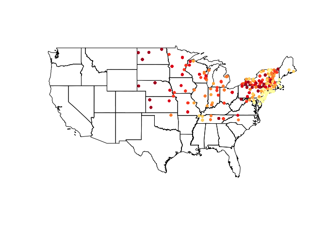
``` r
shades shades$cols plot(us_states)
choropleth(vulgarisSpatial, vulgarisSpatial$Elev,shading = shades, add = T, pch = 20)

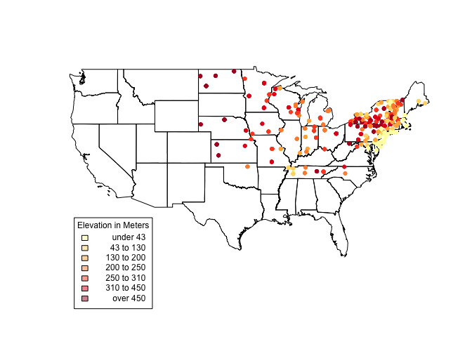
Colors are pretty, but what do they mean? Let’s add a legend.

us_states@bbox #Get us_states bounding box coordinates.

 ##min max
 ## r1 -124.73142 -66.96985
 ## r2 24.95597 49.37173

plot(us_states)
choropleth(vulgarisSpatial, vulgarisSpatial$Elev,shading = shades, add = T, pch = 20)
par(xpd=TRUE) #Allow plotting outside of plot area.
choro.legend(-124, 30, shades, cex = .75, title = "Elevation in Meters") # Plot legend in bottom left. Takes standard legend() params.

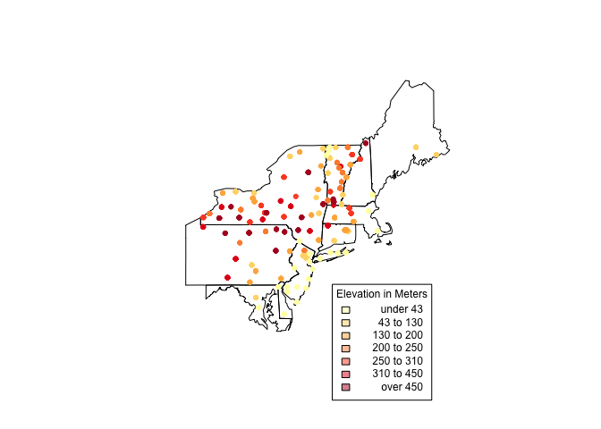
It looks like there’s a lot going on in the Northeastern states. For a
closer look, create another clipping (like above) and plot it. Using the
structure below, we can create a selection vector. I have hidden the
full code since it is repetitive (check GitHub for the full code.)

index '...'

plot(us_states[index,])
choropleth(vulgarisNE, vulgarisNE$Elev,shading = shades, add = T, pch = 20)
par(xpd = T)
choro.legend(-73, 39.75, shades, cex = .75, title = "Elevation in Meters")

Hopefully this has been a useful introduction (or refresher) on spatial
data. I always learn a lot in the process of writing these posts. If you
have any ideas or suggestions please leave a comment or feel free to
contact me!

Happy mapping,

Kiefer