
Recently I have been working on a Kaggle competition where participants are tasked with predicting Russian housing prices. In developing a model for the challenge, I came across a few methods for selecting the best regression
model for a given dataset. Let’s load up some data and take a look.
library(ISLR)
set.seed(123)
swiss <- data.frame(datasets::swiss)
dim(swiss)
## [1] 47 6
head(swiss)
##              Fertility Agriculture Examination Education Catholic
## Courtelary        80.2        17.0          15        12     9.96
## Delemont          83.1        45.1           6         9    84.84
## Franches-Mnt      92.5        39.7           5         5    93.40
## Moutier           85.8        36.5          12         7    33.77
## Neuveville        76.9        43.5          17        15     5.16
## Porrentruy        76.1        35.3           9         7    90.57
##              Infant.Mortality
## Courtelary               22.2
## Delemont                 22.2
## Franches-Mnt             20.2
## Moutier                  20.3
## Neuveville               20.6
## Porrentruy               26.6
This data provides data on Swiss fertility and some socioeconomic
indicators. Suppose we want to predict fertility rate. Each observation
is as a percentage. In order to assess our prediction ability, create
test and training data sets.
index <- sample(nrow(swiss), 5)
train <- swiss[-index,]
test <- swiss[index,]
Next, have a quick look at the data.
par(mfrow=c(2,2))
plot(train$Education, train$Fertility)
plot(train$Catholic, train$Fertility)
plot(train$Infant.Mortality, train$Fertility)
hist(train$Fertility)
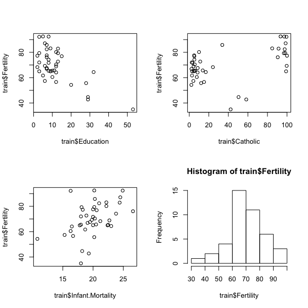
Looks like there could be some interesting relationships here. The
following block of code will take a model formula (or model matrix) and
search for the best combination of predictors.
library(leaps)
leap <- regsubsets(Fertility~., data = train, nbest = 10)
leapsum <- summary(leap)
plot(leap, scale = 'adjr2')

According to the adjusted R-squared value (larger is better), the best
two models are: those with all predictors and all predictors less
Examination. Both have adjusted R-squared values around .69 – a decent fit. Fit these models so we can evaluate them further.
swisslm <- lm(Fertility~., data = train)
swisslm2 <- lm(Fertility~.-Examination, data = train)
#use summary() for a more detailed look.
First we'll compute the mean squared error (MSE).
mean((train$Fertility-predict(swisslm, train))[index]^2)
## [1] 44.21879
mean((train$Fertility-predict(swisslm2, train))[index]^2)
## [1] 36.4982
Looks like the model with all predictors is marginally better. We're
looking for a low value of MSE here. We can also look at the Akaike
information criterion (AIC) for more information. Lower is better here
as well.
library(MASS)
step1 <- stepAIC(swisslm, direction = "both")
step1$anova
## Stepwise Model Path
## Analysis of Deviance Table
##
## Initial Model:
## Fertility ~ Agriculture + Examination + Education + Catholic +
##     Infant.Mortality
##
## Final Model:
## Fertility ~ Agriculture + Education + Catholic + Infant.Mortality
##
##
##            Step Df Deviance Resid. Df Resid. Dev      AIC
## 1                                  36   1746.780 168.5701
## 2 - Examination  1 53.77608        37   1800.556 167.8436
Here, the model without Examination scores lower than the full
model. It seems that both models are evenly matched, though I might be
inclined to use the model without Examination.
Since we sampled our original data to make the train and test datasets,
the difference in these tests is subject to change based on the training
data used. I encourage anyone who wants to test themselves to change the
set.seed at the beginning and evaluate the above results again. Even
better: use your own data!
If you learned something or have questions feel free to leave a comment
or shoot me an email.
Happy modeling,
Kiefer
